Thursday, March 31, 2011

Long EEM Short IWM-How it Works in 3 Ways

Long EEM Short IWM potentially works in 3 ways:

1) See my last post “Asian Currency Opportunity” where currency undervaluation means potential gain of 20-50% versus the US$ and 50%-100% versus the Japanese Yen.  However, even absent the undervaluation, the spread offers protection against a declining dollar, for which most US bond, equity, and real estate investors are not well enough hedged.

2) If the currency undervaluation is not enough, EEM offers better growth at a far lower valuation on an equity basis.  These are not the best indicators of value, but they are public, so I can share them here

Emerging and US Small Cap valuation from Vanguard

Equity characteristics as of 02/28/2011

Emerging Mkts Stk Idx Inv MSCI Emerging Markets Index Net USD

Small-Cap Index Fund Inv

MSCI US Small Cap 1750 Index
Number of stocks 900 796 1722 1716
Median market cap $18.6 billion $18.9 billion $1.8 billion $1.8 billion
price/earnings ratio

14.5x

14.3x

26.1x

26.1x
price/book ratio

2.2x

2.1x

2.1x

2.1x
return on equity

21.70%

21.00%

10.20%

10.20%
earnings growth rate

14.30%

13.70% 3.80% 4.00%

Emerging and US Small Cap valuation stats from iShares EEM and iShares IWM

Fundamentals & Risk as of 2/28/2011
EEM IWM
12-Month Yield 1.41% 1.09%
Price to Earnings Ratio 18.69 27.98
Price to Book Ratio 3.44 3.58

3) The spread offers low correlation versus stocks and bonds in a persistently and dangerously high correlation environment.

From TimelyPortfolio

I’m still not exactly sure how this is calculated, but I thought this offered another look at something statistical, and I feel is not very well covered by other examples.  Points closest to each other on the chart are most related.

From TimelyPortfolio


R code:

require(quantmod)
require(PerformanceAnalytics)
require(fAssets)

tckr<-c("EEM","IEF","IWM","GLD","SPY")

start<-"2005-01-01"
end<- format(Sys.Date(),"%Y-%m-%d") # yyyy-mm-dd

# Pull tckr index data from Yahoo! Finance
getSymbols(tckr, from=start, to=end)

EEM<-adjustOHLC(EEM,use.Adjusted=T)
IEF<-adjustOHLC(IEF,use.Adjusted=T)
IWM<-adjustOHLC(IWM,use.Adjusted=T)
GLD<-adjustOHLC(GLD,use.Adjusted=T)
SPY<-adjustOHLC(SPY,use.Adjusted=T)

EEM<-to.weekly(EEM, indexAt='endof')
IEF<-to.weekly(IEF, indexAt='endof')
IWM<-to.weekly(IWM, indexAt='endof')
GLD<-to.weekly(GLD, indexAt='endof')
SPY<-to.weekly(SPY, indexAt='endof')
EEMIWM<-to.weekly(EEM/IWM, indexAt='endof')

RetToAnalyze<-merge(weeklyReturn(EEM),weeklyReturn(IEF),weeklyReturn(IWM),weeklyReturn(GLD),weeklyReturn(SPY),weeklyReturn(EEMIWM))
colnames(RetToAnalyze)<-c(tckr,"EEMIWM")

assetsDendrogramPlot(as.timeSeries(RetToAnalyze))
assetsCorEigenPlot(as.timeSeries(RetToAnalyze))
mtext("Source: Yahoo! Finance",side=1,adj=0)

chart.Correlation(RetToAnalyze[,1:6,drop=F], main="Correlation since 2005")
mtext("Source: Yahoo! Finance",side=1,adj=0)

#get Rolling Correlations with IEF(bonds) and SPY(stocks)
corEEMIWMtoBonds<-runCor(RetToAnalyze[,6],RetToAnalyze[,2],25)
corEEMIWMtoStocks<-runCor(RetToAnalyze[,6],RetToAnalyze[,5],25)
chartSeries(EEMIWM,TA="addBBands();addTA(corEEMIWMtoBonds);addTA(corEEMIWMtoStocks)",theme="white")
mtext("Source: Yahoo! Finance",side=1,adj=0)


Disclosure:  AS ALWAYS, THESE ARE MY OPINIONS AND THE FUTURE IS UNPREDICTABLE.  CONDITIONS CHANGE AND I ADJUST POTENTIALLY WITHOUT DISCLOSURE ON THIS BLOG.  YOU ARE ON YOUR OWN MAKING INVESTMENT DECISIONS, AND IN NO WAY AM I ADVISING YOU.  I TAKE NO RESPONSIBILITY FOR YOUR GAINS OR LOSSES.

Asian Currency Opportunity

Asian currencies are fundamentally undervalued at an extreme level due to the Central Banks’ focus on the US$.  For those that regularly read my blog or happened to see me in SmartMoney, this will not surprise you,

“And investors can also buy emerging-market stocks in countries whose currencies appear undervalued, potentially seeing double gains from currency appreciation and stock price growth, Russell says.”

At this point, I have no idea where the stock markets of the world go, but fortunately, I do not need to care, since I am not an equity manager.  However, my best method of pursuing Asian currencies comes through emerging market equity etfs, so if I buy EWY Ishares Korea, I am also buying the Korean Won and shorting the US$.  I like all the Asian emerging currencies, but for this post want to focus on the Korean Won to avoid any additional confusion.  See my post Japan Intentional or Accidental Pursuit of Deflation for more in depth discussion of all the Asian emerging currencies.

Yesterday, three years from the 2007-2008 disaster and almost a year from the Flash Crash, the heavens seem to have opened and the skies seem to have cleared for the Korean Won vs the US$, Japanese Yen, and Euro. 

From TimelyPortfolio

All of the potential currency profits that have so far been untapped from EWY now seem a real possibility,


via StockCharts.com

but if you’re like me and uncertain about the next direction of equity markets, then a spread trade with EWY long and IWM short can ease your equity fears.  However, feel free to blend the spread to your tastes.  I like to add a little short Japanese Yen.


via StockCharts.com

R code:

require(quantmod)
require(PerformanceAnalytics)

#get asian currency data from the FED FRED data series
getSymbols("DEXKOUS",src="FRED") #load Korea
getSymbols("DEXJPUS",src="FRED") #load Japan

#other symbol options
#getSymbols("DEXMAUS",src="FRED") #load Malaysia
#getSymbols("DEXSIUS",src="FRED") #load Singapore
#getSymbols("DEXTAUS",src="FRED") #load Taiwan
#getSymbols("DEXCHUS",src="FRED") #load China

#invert to get KRWUSD and JPYUSD
asian<-merge(1/DEXKOUS,1/DEXJPUS)

#do dailyReturn so that I can use pretty PerformanceAnalytics charts
#division puts currencies in Japanese yen from US dollar
asianreturn<-merge(dailyReturn(asian[,1]),dailyReturn(asian[,1]/asian[,2]))

#label columns for graph legends
colnames(asianreturn)<-c("KoreaUS","KoreaJapan")

chart.CumReturns(asianreturn["2007::2011"],legend.loc="right",main="Korean Won in US$ and Japanese Yen",ylab="")
mtext("Source: Federal Reserve FRED",side=1,adj=0)


Disclosure:  AS ALWAYS, THESE ARE MY OPINIONS AND THE FUTURE IS UNPREDICTABLE.  CONDITIONS CHANGE AND I ADJUST POTENTIALLY WITHOUT DISCLOSURE ON THIS BLOG.  YOU ARE ON YOUR OWN MAKING INVESTMENT DECISIONS, AND IN NO WAY AM I ADVISING YOU.  I TAKE NO RESPONSIBILITY FOR YOUR GAINS OR LOSSES.

Tuesday, March 29, 2011

The Leverage Space Trading Model

I finally got around to reading Ralph Vince’s latest The Leverage Space Trading Model (for a brief summary see this magazine article in Futures), and I’m happy to say that the book was very helpful in approach and example.  I especially enjoyed the last two chapters which tied his method to the realities of the money management business which do not fit most economic models.

The book’s true value will reveal itself hopefully through my ability to incorporate the material.  As usual with R, some fine folks at http://www.fosstrading.com and http://automated-trading-system.com have already built a package and provided examples on its use.  To extend their examples, I wanted to apply this Leverage Space Model to the EDHEC Hedge Fund Returns provided in the PerformanceAnalytics R package and then use this PerformanceAnalytics package to produce some decent charts illustrating the output.

From TimelyPortfolio

Since the book uses $ amounts instead of percentages, I am not entirely sure I got this correct, but it is certainly close.  As always, please let me know if I messed up here or anywhere.

After your comments and my own improvements, I hope to extend this to basic systems and show how we can tie multiple managers, systems, or indicies together with the Leverage Space approach.  Also, I would like to compare this with other optimization methods to see which are more robust.


R code:

#Please see au.tra.sy blog http://www.automated-trading-system.com/
#for original code and http://www.fosstrading.com
#I take no credit for the majority of this code
#I simply changed a couple of things to use edhec data
#as another example but this time using xts style returns

require(PerformanceAnalytics)

# Set Walk-Forward parameters (number of periods)
optim<-48 #4 years = 48 monthly returns
wf<-6 #walk forward 6 monthly returns
# get data series from PerformanceAnalytics edhec dataset
data(edhec)
rtn<-edhec[,1:13]*100
# Calculate number of WF cycles
numCycles = floor((nrow(rtn)-optim)/wf)
# Define JPT function
jointProbTable <- function(x, n=3, FUN=median, ...) {
  # Load LSPM
  if(!require(LSPM,quietly=TRUE)) stop(warnings())
  # Function to bin data
  quantize <- function(x, n, FUN=median, ...) {
    if(is.character(FUN)) FUN <- get(FUN)
    bins <- cut(x, n, labels=FALSE)
    res <- sapply(1:NROW(x), function(i) FUN(x[bins==bins[i]], ...))
  }
  # Allow for different values of 'n' for each system in 'x'
  if(NROW(n)==1) {
    n <- rep(n,NCOL(x))
  } else
  if(NROW(n)!=NCOL(x)) stop("invalid 'n'")
  # Bin data in 'x'
  qd <- sapply(1:NCOL(x), function(i) quantize(x[,i],n=n[i],FUN=FUN,...))
  # Aggregate probabilities
  probs <- rep(1/NROW(x),NROW(x))
  res <- aggregate(probs, by=lapply(1:NCOL(qd), function(i) qd[,i]), sum)
  # Clean up output, return lsp object
  colnames(res) <- colnames(x)
  res <- lsp(res[,1:NCOL(x)],res[,NCOL(res)])
  return(res)
}
for (i in 0:(numCycles-1)) {
            # Define cycle boundaries
            start<-1+(i*wf)
            end<-optim+(i*wf)
            # Get returns for optimization cycle and create the JPT
            jpt <- jointProbTable(rtn[start:end],n=rep(10,13))
            outcomes<-jpt[[1]]
            probs<-jpt[[2]]
            port<-lsp(outcomes,probs)
            # DEoptim parameters (see ?DEoptim)
            np=130       # 10 * number of mktsys
            imax=1000       #maximum number of iterations
            crossover=0.6       #probability of crossover
            NR <- NROW(port$f)
            DEctrl <- list(NP=np, itermax=imax, CR=crossover, trace=TRUE)
            # Optimize f
            res <- optimalf(port, control=DEctrl)
        # use upper to restrict to a level that you might feel comfortable
            #res <- optimalf(port, control=DEctrl, lower=rep(0,13), upper=rep(0.2,13))

    # these are other possibilities but I gave up after 24 hours
        #maxProbProfit from Foss Trading
        #res<-maxProbProfit(port, 1e-6, 6, probDrawdown, 0.1, DD=0.2, control=DEctrl)
        #probDrawdown from Foss Trading
        #res<-optimalf(port,probDrawdown,0.1,DD=0.2,horizon=6,control=DEctrl)

            # Save leverage amounts as optimal f
        # Examples in the book Ralph Vince Leverage Space Trading Model
        # all in dollar terms which confuses me
        # until I resolve I changed lev line to show optimal f output
            lev<-res$f[1:13]
            levmat<-c(rep(1,wf)) %o% lev #so that we can multiply with the wfrtn
            # Get the returns for the next Walk-Forward period
            wfrtn <- rtn[(end+1):(end+wf)]/100
            wflevrtn <- wfrtn*levmat #apply leverage to the returns
            if (i==0) fullrtns<-wflevrtn else fullrtns<-rbind(fullrtns,wflevrtn)
        if (i==0) levered<-levmat else levered<-rbind(levered,levmat)
}

#not super familiar with xts, but this add dates to levered from the wflevrtn xts series
levered<-xts(levered,order.by=index(fullrtns) )
chart.StackedBar(levered, cex.legend=0.6)

#just the first six in the series as another example
#I had to fill the window to my screen to avoid a error from R on margins
par(mfrow=c(6,1))
for (i in 1:6) {
chart.TimeSeries(levered[,i],xlab=NULL)
}

charts.PerformanceSummary(fullrtns, main="Performance Summary with Optimal f Applied")

Tuesday, March 22, 2011

Free and Easy Currency Monitor in R

Certainly not the best way to keep up with currencies, but the increasingly important job of monitoring currencies can be free and easy in R using Federal Reserve FRED data.  Here is a template that can be adjusted to your favorite currencies with symbols listed here.

See my previous post on how to monitor the potential US Dollar Collapse cheaply and easily.  Also, currencies are important again, so do not ignore them when investing.  Don’t say I did not warn you and don’t make excuses that you don’t have expensive gear.

From TimelyPortfolio

R code:

require(quantmod)
require(PerformanceAnalytics)

#get asian currency data from the FED FRED data series
getSymbols("DEXKOUS",src="FRED") #load Korea
getSymbols("DEXMAUS",src="FRED") #load Malaysia
getSymbols("DEXSIUS",src="FRED") #load Singapore
getSymbols("DEXTAUS",src="FRED") #load Taiwan
getSymbols("DEXCHUS",src="FRED") #load China
getSymbols("DEXJPUS",src="FRED") #load Japan
getSymbols("DEXTHUS",src="FRED") #load Thailand
getSymbols("DEXBZUS",src="FRED") #load Brazil
getSymbols("DEXMXUS",src="FRED") #load Mexico
getSymbols("DEXINUS",src="FRED") #load India
getSymbols("DTWEXO",src="FRED") #load US Dollar Other Trading Partners
getSymbols("DTWEXB",src="FRED") #load US Dollar Broad

par(mfrow=c(3, 4)) #provides 4 columns and 3 rows for charts
plot(1/coredata(DEXKOUS["1995::2011"]),type="l",ylab="Korea")
plot(1/coredata(DEXMAUS["1995::2011"]),type="l",ylab="Malaysia")
plot(1/coredata(DEXSIUS["1995::2011"]),type="l",ylab="Singapore")
plot(1/coredata(DEXTAUS["1995::2011"]),type="l",ylab="Taiwan")
plot(1/coredata(DEXCHUS["1995::2011"]),type="l",ylab="China")
plot(1/coredata(DEXJPUS["1995::2011"]),type="l",ylab="Japan")
plot(1/coredata(DEXTHUS["1995::2011"]),type="l",ylab="Thailand")
plot(1/coredata(DEXBZUS["1995::2011"]),type="l",ylab="Brazil")
plot(1/coredata(DEXMXUS["1995::2011"]),type="l",ylab="Mexico")
plot(1/coredata(DEXINUS["1995::2011"]),type="l",ylab="India")
plot(coredata(DTWEXO["1995::2011"]),type="l",ylab="US Dollar Other")
plot(coredata(DTWEXB["1995::2011"]),type="l",ylab="US Dollar Broad")

#if you prefer a prettier chart then you can use
chartSeries(to.monthly(1/DEXSIUS),theme = chartTheme("white"),name="Singapore Dollar/USD",TA="addBBands(10)")

Thursday, March 17, 2011

Japanese Government Bonds for 3bps-Come and Get It

For those readers that want data not my thoughts, here is something courtesy of Bloomberg that is not generally discussed or shown.  If you buy the Japan 10 year and hedge credit risk, you get a maximum 3 bps return each year for the next 10 years.

From TimelyPortfolio

Why Talk My Book?

Gray, Wesley R. and Kern, Andrew E., Talking Your Book: Social Networks and Price Discovery (February 22, 2011). Available at SSRN: http://ssrn.com/abstract=1767452 explores the outperformance of ideas posted on the Value Investors Club site.  I enjoyed this article more for the exploration and summary of research on their “Talk Your Book (TYB)” model than the analysis of outperformance.  The discussion of TYB gives me a good chance to explore the reasons I blog or talk my book, which is not the same as their model suggests:

A simple example illustrates how investors utilize TYB in the marketplace. Consider a fund manager who, on the basis of her private information, identifies a stock that is selling for 50% of its intrinsic value. The manager will deploy her capital to the fullest extent possible, stopping only when her capital base is exhausted or she reaches a mandated portfolio position
risk limit (e.g., 10% of net asset value). Notwithstanding the price pressure exerted by the manager herself, the stock may remain considerably undervalued. Because the fund manager has no further ability to increase the size of her position, she faces limited costs in sharing her information. She therefore shares her private information with other arbitrageurs in her social network. These other arbitrageurs verify the private information and, by deploying capital of their own, ultimately drive the price of the asset closer to intrinsic value.


TYB benefits all parties involved: The sharer experiences a gain as her portfolio increases in value, the arbitrageurs who receive the shared information obtain access to a profitable trading opportunity, and prices slowly approach intrinsic value. In the end, prices reach intrinsic value, but market efficiency is a multi-stage process because information must travel through a social network before it is fully reflected in asset prices.

I blog to

1) record my thoughts with a timestamp and no benefit of hindsight

2) improve the thoroughness of my thoughts through the Hawthorne Effect.  If I publish something for all the world to see, I am going to make absolute sure that my references are correct.

3) get feedback to improve my thoughts.  Please criticize and bash what I write.  The markets hurt my feelings all the time and do far more damage than your thoughts ever will.  Please share them.

Markets have humbled me far too greatly to believe that I can or will move markets.  Only the established trend of the market can attract enough attention to move the market meaningfully in my favor.  Markets are not efficient, and I have no private information.  I simply need to be an diligent, honest, and humble observer of the market, and I will do well.

Fat-tailed Events Should Lead to Fat-tailed Market Action

I’m deeply sympathetic to the extreme tragedy in Japan.  The human loss and damage troubles me and makes focusing on markets unusually difficult.  So far, I have determined that the pricing mechanism of free markets has failed miserably over the last week.  Fat-tailed events in the most connected country in the world should lead to a fat-tailed market response.  If we all knew what was going to happen this week last week, most of us would have lost money.  Panic in markets?  What panic?  Russell 2000 down 1.5% for the week and S&P 500 down 2.5% does not even incorporate the news we know much less the extreme uncertainty left by the silent unknown and potential bad case.  I have not seen markets pricing in the best case in all my market experience and extensive study.

Japanese CDS are at 117 bps and the JGB 10y offers 119 bps.  2 bps compensation for a potential loss of 2000 bps or more just does not make any sense.

The market will see a fat-tailed response in far more ways than the Yen and Nikkei.  Markets experience fat-tailed distributions even without fat-tailed events, so I do not think this a grand assumption.  The calamity is a fat-tailed events and will lead to far more significant consequences than we have experienced over the past couple of days.

Thursday, March 10, 2011

Absurdly Illogical-Gross Sells Treasuries to be Long US Dollar-What???

I saw this and at first thought Bill Gross made comments alluding to this.  However, it is just an illogical and somewhat absurd analysis of his remarks.

    Why Is Bill Gross Betting On A Vicious Move Higher In The Dollar?

    businessinsider

    Joe Weisenthal, On Thursday March 10, 2011, 7:05 am EST

    Yesterday PIMCO reported that it had completely abandoned US government bonds.

    Perhaps more importantly, PIMCO now has a gigantic position in cash -- it's biggest ever.

    Is PIMCO betting on a vicious rally in the dollar?

    There are a few reasons it could happen:

    • The crackup of the Eurozone will help the dollar.
    • The end of QEIII is looking more and more likely.
    • Anti-dollar sentiment is extreme.
    • Commodities are all looking peakish, etc.
    • Aggressive spending cuts in DC.

    The signs are building up.

    Unfortunately, I had to do something I don’t like to do to find out--read his outlook.  In it, he states

    An inflation-adjusted “negative buck” might be more likely.

    which I interpret to mean losses on interest rates and the US dollar.

    If (and I think a hugely doubtful if this time around) the US maintains the status quo with the dollar as reserve currency for the world, then all of the events listed below incite a rally in US Treasuries, in which Bill Gross would want to participate.  Neither Bill Gross nor his fund receive any benefit from being long a US dollar, since he and his clients are already implicitly long the dollar and he is measured by US bonds.  Selling US Treasuries and holding US dollars as cash implies a belief that US interest rates move higher.  What most likely causes US interest rates to move higher are inflation through higher commodity prices, continued stimulative and aggressive monetary policy, and/or abandonment of the US dollar as a reserve currency.  However, strangely enough, each of those reasons leads to the other two.  Monetary policy is inflationary and leads to higher rates and eventual loss of confidence in the Fed and abandonment of the US dollar as reserve currency; and similarly but in reverse inflation through higher commodity prices causes Emerging Asia to rectify their undervalued currencies by selling US Treasuries and US dollars but does nothing to stop Ben Bernanke and Fed policy.

    The Fed has lost its ability to be lender of last resort, so now the lender of last resort is emerging Asia.

    US interest rates and really everything are entirely dependent on the US dollar as a reserve currency in an imbalanced and vulnerable global situation.  The only thing that fixes these imbalances are lower US dollar and higher rates, and we do not get one without the other, and we don’t get any without some considerable pain.  I always shutter when I hear “This time is different,” so let me be clear,

    last time 2007-2009 was different

    and what happens next will be the same as all of recorded financial history as the US finds the limits to its monetary and fiscal policy.

    Now, the real question is what reserve currency fails first and faces speculative attack.  If it is the Euro, then the US dollar probably rallies, and we’re stuck in an imbalanced system.  If it is the British Pound or Japanese Yen, then the first line of defense will be to sell the US dollar and US Treasuries, which then leads to a domino effect and US dollar failure.  If it is the US dollar, then I don’t know what to do except be short everything except Emerging Asian currencies and potentially the only thing of value in the US (agricultural commodities).

    I feel very fortunate to be a US citizen, but I have also resolved to not let my citizenry blind my investment policy and implicitly get me even more leveraged to the US dollar.  US investors do not have to face the same fate as US citizens.

    Friday, March 4, 2011

    Nine Lives of the Fed Put

    Are we at the 9th life of the Fed (Greenspan) put?

    1) 1987-Black Monday

    2) 1992-S&L

    3) 1994-Mexico

    4) 1998-LTCM and Russia

    5) 2000-2002 Tech Bubble Collapse

    6) 2008-AIG, FNMA, FHLMC and all other financial institutions except Lehman

    7) 2009-QE1

    8) 2010-QEII

    9) Response to next crisis

    Unsustainable Gift

    Reflecting on my previous post, I feel like we have all been given an incredible gift over the last two years that is completely unsustainable.  Any investor/speculator that has benefitted from that gift should recognize its existence first and its potential expiration second.  Cognitive dissonance at this point might lead to a “Master of the Universe” feeling right now even though none of us have had control over the decisions or $10 trillion that got us here.  Be grateful for your profits but protect them from the reverse as we approach the limits of our policies.  Santa comes once a year, but Bernanke and emerging reserves of $10 trillion come once in a lifetime.

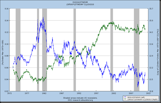
    Death Spiral Warning Graph

    In the death spiral scenario, rates go up while the currency goes down.  Here is the way to watch that.  I’m not saying that death spiral of US Dollar and interest rates occurs, but without significant action to restore confidence in fiscal and monetary policies, it is almost certain.  Fortunately free markets and a democracy might stop the spiral early, but it appears a mini-crisis is necessary to force action.

    via StockCharts.com

    And when we add this as the denominator or pricing mechanism for the S&P 500 (transformation requires removing natural $ pricing first), the chart looks like this.  The transitory fake improvement in stock prices since 2008 driven by aggressive monetary action is much clearer.  Anything through 14.3 on the green line is indicative of the first phase of this spiral.

     fed fred rates dollar sp500

    And to throw a little R into this, let’s look at the rolling correlation of the SP500 to the 10y/US$ ratio.  The correlation magically increases in Summer 1998 with Long Term Capital Management and Russia default, and the Fed put became entrenched.

    From TimelyPortfolio


    R code:

    require(quantmod)
    require(PerformanceAnalytics)

    #get currency rate and stock data from the FED FRED data series
    getSymbols("DGS10",src="FRED") #load Fed 10y rate
    getSymbols("DTWEXM",src="FRED") #load Fed Dollar
    getSymbols("DTWEXO",src="FRED") #load Fed Dollar Other
    getSymbols("SP500",src="FRED") #load Fed SP500

    returns<-merge(monthlyReturn(to.monthly(DGS10/DTWEXM)),monthlyReturn(to.monthly(SP500)))

    corSP10USD<-runCor(returns["1973::2011-02",1],returns["1973::2011-02",2],n=6)

    chartSeries(corSP10USD,theme='white',name="S&P 500 Rolling 1y Correlation with US$ and US10y Rates")

    Wednesday, March 2, 2011

    Death Spiral of a Country

    I have spent considerable time studying rapid collapses of nations or regions.  Below is a crude summary of what I have so far assimilated.

    image

    What concerns me most about reaching the limits of fiscal and monetary stimulus is the inability to respond in the next crisis as the US Dollar falls, US rates increase, and US stocks plummet.  This is the positive feedback loop in a negative cycle that was disrupted in 2007-2008 as the Dollar increased due its reserve currency status.  Dollar stability also allowed rates to decrease precipitously and the Fed and Congress to engage in actions that otherwise would not have been available.

    What I have not determined is the general chronology of the losses in a death spiral.  It seems rates move up, stocks move down, and then confidence erodes and the real damage begins.

    Tuesday, March 1, 2011

    R User Group Birmingham Alabama

    I would like to start a R user group in Birmingham, Alabama.  Please comment if anyone is interested.  I’m thinking I will host in Google Groups, since meetup costs money.  Let me know if I should use some other site.

    Since My Barron’s Debut

    Jack Willoughby in Barron’s November 1, 2010 summarized their Big Money Poll in an article titled “Bears Beware.”  Commenters on Twitter and blogs everywhere cited this as a perfect “Cover Story” indicator to exit the stock market.  This article was also my Barron’s debut

    "Bonds aren't the best place to make money," says Kenton Russell, a portfolio manager for Sterne Agee. "They are severely overvalued. The only way a bond investment works at current yields is if we're in a depression. Some ugly things [would] have to come true."

    Russell recommends high-yielding, big-cap stocks issued by companies with strong balance sheets. The most bullish Big Money participant, he predicts the Dow will reach 14,000 by mid-2011, with the S&P rising to 1,300 and the Nasdaq to 2,500. Investors have abandoned risk "precisely at the time they should be taking risks," he says.

    I hope I am this right every time I appear in Barron’s as seen in the chart below

    via StockCharts.com

    Unfortunately though, I think the move in stocks is almost done just as my targets are reached 5 months early, so I’m not sure it counts.  I would love to see the poll now.  My guess is it would be much different with many more aggressive bulls and with me as a bear.